Instantaneous Velocity Calculator: Finding Velocity at a Single Moment With the Derivative
Here's a question that sounds like a trick but isn't: how can a car have a speed at the exact instant your stopwatch reads 3.000 seconds? Speed is distance over time, and a single instant has no duration — zero seconds of elapsed time. Divide any distance by zero and the math falls apart. Yet your speedometer cheerfully displays a number at every moment. Instantaneous velocity is the physics that resolves that paradox, and this calculator computes it the honest way: by taking the derivative of a position function, which is exactly the limit of Δx/Δt as the interval shrinks toward — but never reaches — zero.
How Can Velocity Exist at a Single Instant?
The way out of the paradox is to stop demanding an answer at a literal zero-width instant and instead ask what value the average velocity is heading toward as you measure over smaller and smaller windows. Take a ball whose position follows x(t) = 5t². Measure its average velocity from t = 2 s over the next full second and you get (5·3² − 5·2²)/1 = 25 m/s. Shrink the window to 0.1 s and the average climbs to 20.5 m/s. Shrink it to 0.01 s and you land on 20.05 m/s. The numbers aren't wandering randomly — they're homing in on 20 m/s, and that target they approach is the instantaneous velocity at t = 2.
Notice that none of those windows ever had a width of zero. We never divided by nothing. We watched a trend and read off where it was obviously going. That sleight of hand — getting an answer "at a point" without ever plugging in a zero interval — is the single idea behind every derivative in calculus, and instantaneous velocity is where most students meet it for the first time.
Instantaneous Velocity Is the Limit of Δx/Δt
Written formally, instantaneous velocity is v = limΔt→0Δx/Δt, which is the definition of the derivative dx/dt. The notation looks intimidating, but it's just shorthand for the squeezing process from the last section. The average velocity gives you Δx/Δt over a finite chunk of time; the instantaneous velocity is the number that average converges to as the chunk vanishes. This is why the two are equal only when velocity never changes — a constant function is its own limit.
The calculator above runs this limit live. Type any position function and it evaluates the forward average (over [t, t+Δt]) and the backward average (over [t−Δt, t]) for Δt = 1, 0.1, 0.01, and 0.001. You'll see both columns clamp down on the same value from opposite sides. When a forward average overshoots and a backward average undershoots — or vice versa — the true instantaneous velocity is pinned between them, and each tenfold shrink in Δt buys you roughly one more matching digit.
Watching the Limit Close In on the Answer
Convergence isn't just a formality; the rate of it tells you something physical. For the smooth function x(t) = 5t² + 3t at t = 2 s, the averages converge on 23 m/s quickly because the curve is gentle there. Feed in an oscillation like x(t) = 3·sin(2t) and the same Δt values converge more slowly near a sharp turning point, because the curve is bending fast and a finite Δt straddles more of that bend. The table below tracks x(t) = 5t² + 3t at t = 2 s, where the exact answer is v = 10·2 + 3 = 23 m/s.
| Interval width Δt | Average over [2, 2+Δt] (m/s) | Error from 23 m/s |
|---|---|---|
| 1.0 s | 28.0 | +5.0 |
| 0.1 s | 23.5 | +0.5 |
| 0.01 s | 23.05 | +0.05 |
| 0.001 s | 23.005 | +0.005 |
Every time Δt drops by a factor of 10, the error drops by the same factor — a dead-straight march toward 23 m/s. That linear shrink is the fingerprint of a forward difference on a smooth curve. The exact derivative skips all of it and hands you 23 m/s in one step, which is why physicists reach for the rule rather than a table once they trust where the limit lands.
The Tangent Line: A Slope at a Single Point
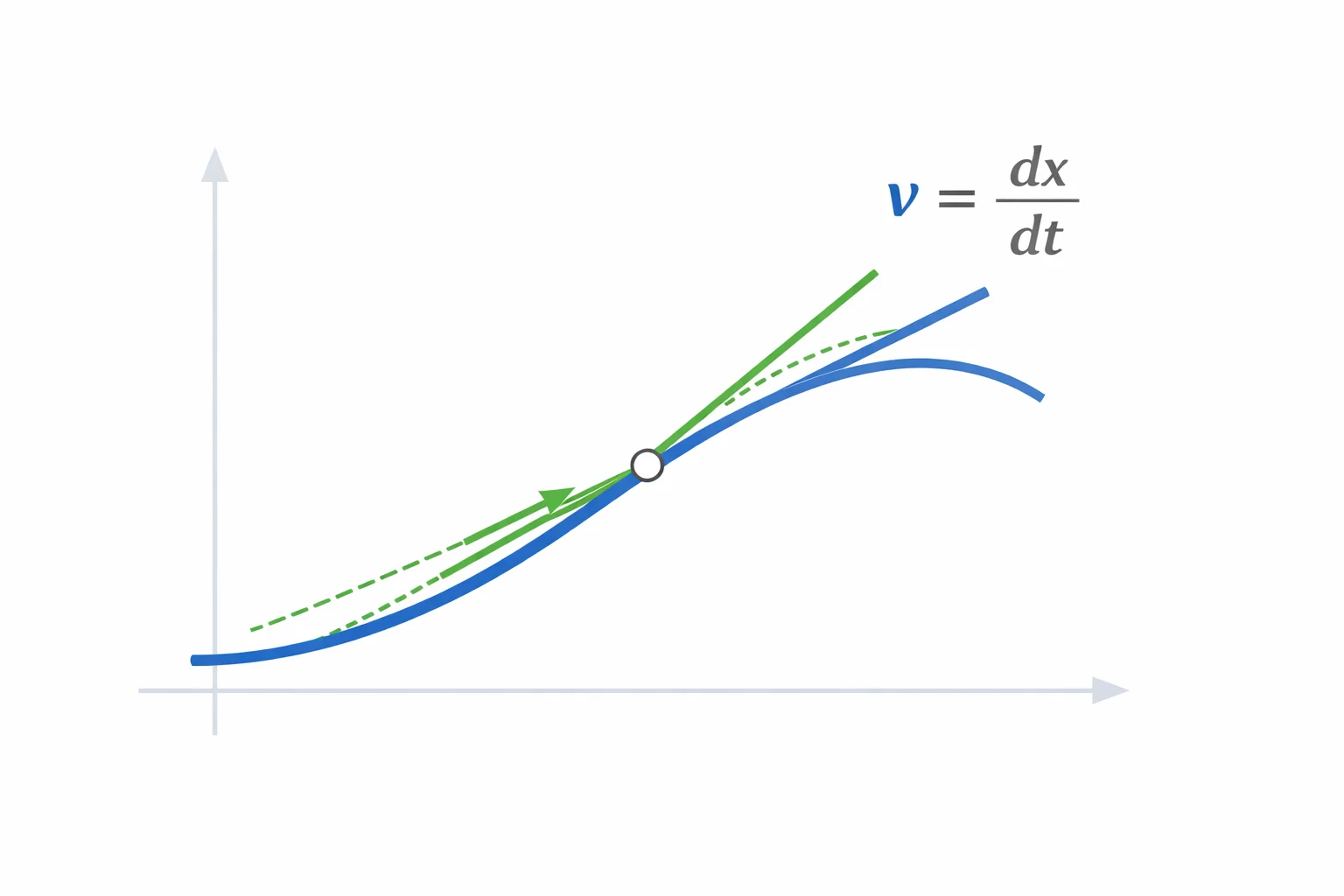
Geometrically, every average velocity is the slope of a secant line — the straight line cutting through two points on a position-time graph. As those two points slide toward each other, the secant pivots, and in the limit it becomes the tangent: the line that just grazes the curve at one point. The slope of that tangent is the instantaneous velocity. This is the same secant-to-tangent collapse you can read off a slope of a graph calculator, just applied to motion data.
That picture explains a fact students often memorize without understanding: a horizontal tangent means zero velocity. When a ball thrown upward reaches the top of its arc, its position-time graph flattens into a momentary horizontal tangent, so v = 0 there — even though gravity is still pulling at 9.8 m/s² the entire time. The calculator reports that acceleration separately as the second derivative, so you can watch velocity pass through zero while acceleration stays put.
The Power Rule Turns Position Into Velocity
For any position written as a power of t, one rule does all the work: the derivative of tn is n·tn−1. Multiply each term by its exponent, then knock the exponent down by one. So x(t) = 5t² becomes v(t) = 10t, a constant out front carries along, and any standalone constant — your starting position — differentiates to zero because it doesn't change with time. That last point is worth underlining: where the object startsnever affects how fast it's moving.
Constant-acceleration motion is the case you'll meet most. Its position function is x(t) = x₀ + v₀t + ½at², and the power rule differentiates it term by term into v(t) = v₀ + at — the familiar kinematic equation, derived rather than memorized. The ½at² becomes at, and the constant x₀ vanishes. Differentiate once more and you recover the constant acceleration a, which is precisely why a quadratic position means a steady acceleration and a cubic position means an acceleration that itself changes over time.
Worked Example: A Rocket With Changing Acceleration
Suppose a model rocket's height during burn follows x(t) = t³ − 6t² + 20t meters for the first few seconds, where the cubic term captures a motor whose thrust isn't steady. What's its instantaneous velocity at t = 3 s? Apply the power rule to each term: the derivative is v(t) = 3t² − 12t + 20. Now substitute: v(3) = 3·9 − 12·3 + 20 = 27 − 36 + 20 = 11 m/s. The rocket is climbing at 11 m/s at that instant.
Push it further and the cubic earns its keep. The acceleration is the derivative of velocity, a(t) = 6t − 12, so at t = 3 s the rocket accelerates at 6·3 − 12 = 6 m/s². But rewind to t = 1 s and a(1) = 6 − 12 = −6 m/s² — the rocket was decelerating early in the burn and only later began gaining acceleration. A single quadratic-position model could never show that reversal; you need the cubic, and you need the derivative to extract the velocity at each instant. Drop this exact function into the calculator at different times to trace the whole flight profile.
Speedometer vs Trip Odometer: Two Kinds of Velocity
The cleanest way to keep instantaneous and average velocity straight is the dashboard analogy. Your speedometer reads instantaneous velocity — how fast you're going right now, this instant. Your trip computer's "average speed" readout divides total displacement by total elapsed time, an average velocity over the whole drive. On a road trip with stoplights and a highway stretch, those two numbers can disagree wildly.
| Property | Instantaneous velocity | Average velocity |
|---|---|---|
| What it measures | Velocity at one instant | Velocity over an interval |
| Math operation | Derivative dx/dt (a limit) | Division Δx/Δt |
| Graph reading | Slope of the tangent line | Slope of the secant line |
| Dashboard match | Speedometer needle | Trip computer average |
They coincide in exactly one situation: constant velocity. If the speedometer never moves, the average over any stretch equals that fixed reading, and the position-time graph is a straight line whose every tangent has the same slope as its secants. The moment the motion accelerates, the two split — and which one a problem wants is usually the whole point of the question.
Where the Tangent Trick Trips Students Up
- Confusing zero velocity with zero acceleration. At the top of a toss, v = 0 but a = −9.8 m/s². The object is momentarily still yet still being pulled. A horizontal tangent on the position graph never implies a flat velocity graph.
- Plugging Δt = 0 into Δx/Δt.You can't — that's 0/0, undefined. The limit and the derivative exist precisely to get the answer without that illegal division. Always differentiate or take the limit; never substitute zero directly.
- Differentiating the constant term. The starting position x₀ has derivative zero, so it never appears in the velocity. A ball dropped from 80 m and one dropped from 200 m have identical velocity functions — the height only sets where the motion begins.
- Reading speed off a negative velocity. A velocity of −12 m/s has a speed of 12 m/s; the minus sign is direction. Reporting the instantaneous speed as −12 throws away exactly the directional information instantaneous velocity is built to carry.