Area Under a Curve Calculator: How to Integrate Physics Graphs for Real Quantities
A speedometer never tells you how far you've driven. It only ever shows your speed right now. Yet if you sketched your speed against time for a whole trip and shaded in everything underneath that line, the area of the shaded region would be the exact distance you covered. That is the whole idea behind the area under a curve: it converts a rate you can read at any instant into the total amount that accumulated. An area under a curve calculator does that conversion for any physics graph you throw at it — turning velocity into displacement, force into work, current into charge.
The Area Is the Total, Not the Rate
Here's the cleanest way to see why area gives a total. Take a flat velocity-time graph where a car holds a steady 20 m/s for 8 seconds. The region under the line is a rectangle: 20 m/s tall and 8 s wide. Its area is 20 × 8 = 160, and the units multiply too — (m/s) × s = m. So the area is 160 metres, which is exactly how far the car travelled. The graph never printed “160 m” anywhere, but it was sitting there as an area the whole time.
The reason this matters is that the slope and the area pull two completely different numbers off the same line. Slope divides the axes and gives you a rate; area multiplies them and gives you an accumulated total. On a velocity-time graph the slope is acceleration in m/s², while the area is displacement in metres. If you want the steepness reading instead, the slope of a graph calculator handles that side; this tool is built for everything the area tells you.
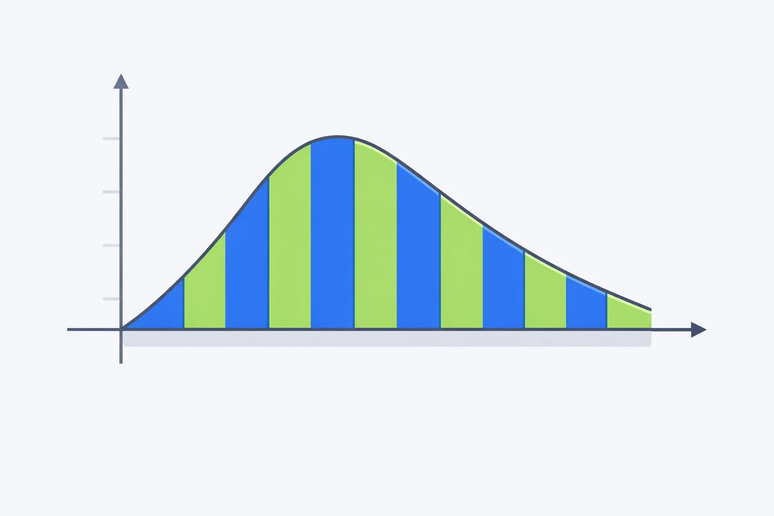
The Trapezoidal Rule: Strips You Can Add Up
Real graphs are rarely a single clean rectangle. The trick is to chop the area into thin vertical strips, work out the area of each one, and add them. When you connect two neighbouring data points with a straight segment, the strip beneath becomes a trapezoid, and a trapezoid's area is its average height times its width: ½·(y₁ + y₂)·Δx. That's the trapezoidal rule, and it's what the calculator sums across your whole data set.
Suppose two readings on a velocity-time graph are 14 m/s at t = 2 s and 20 m/s at t = 3 s. The strip between them is ½·(14 + 20)·1 = 17 metres. Do that for every neighbouring pair and the running total is the displacement. Notice the rule never assumes the points lie on a straight line overall — it follows the real curve segment by segment, which is why it copes with data that bends.
Worked Example: Displacement From a Velocity-Time Graph
Take the calculator's default data — a car pulling away from a junction, its velocity logged each second: 0, 6, 14, 20, 24, and 25 m/s at t = 0 through 5 s. The curve is steep at first and flattens as the car approaches its cruising speed, exactly the shape of real acceleration. We want the distance covered.
Add the five trapezoidal strips: ½·(0+6)·1 = 3, then 10, 17, 22, and 24.5 metres. The total is 76.5 m. That's the displacement over five seconds — and it came purely from the area, no kinematics equation in sight. Now look at the bracketing: the left-rectangle sum (using the lower velocity in each strip) gives 64 m, and the right-rectangle sum gives 89 m. The trapezoid's 76.5 m sits dead centre between them, because a trapezoid is just the average of the two rectangles. The true area has to lie between an under-estimate and an over-estimate, which is a handy sanity check the calculator gives you for free.
Rectangles, Trapezoids, Simpson: Which Method and How Wrong
The calculator shows several estimates at once because no single numerical method is always best. Each one approximates the strips differently, and knowing how each one fails tells you which number to trust:
| Method | How it fills a strip | Tends to | Exact when the curve is |
|---|---|---|---|
| Left rectangle | Flat top at the left height | Under-estimate on a rising curve | Horizontal |
| Right rectangle | Flat top at the right height | Over-estimate on a rising curve | Horizontal |
| Trapezoidal | Sloped top joining both heights | Slight over-estimate on a curve bowing up | A straight line |
| Simpson's rule | Parabola through three points | Very small error on smooth curves | A parabola (or cubic) |
Simpson's rule is the quiet star here. Instead of straight-line tops it fits a parabola through each trio of points, so it matches any data that genuinely curves — projectile motion, a charging capacitor, a quadratic velocity profile — far better than the trapezoid for the same number of points. The trade-off is that it demands equally spaced x-values and an even number of intervals, which is why the calculator only displays the Simpson figure when your data qualifies. When it does appear and differs noticeably from the trapezoid, trust Simpson on a smooth curve.
What the Area Becomes on Each Physics Graph
The arithmetic of the trapezoidal rule never changes — only the physical meaning does, because the axis units change. Every row below is an integral pairing worth knowing, and switching the graph type in the calculator relabels everything for you:
| Graph (y vs x) | Area equals | Matches | Unit |
|---|---|---|---|
| Velocity vs time | Displacement | s = v·t | m |
| Acceleration vs time | Change in velocity | Δv = a·t | m/s |
| Force vs displacement | Work done | W = F·s | J |
| Force vs time | Impulse | J = F·t | N·s |
| Power vs time | Energy transferred | E = P·t | J |
| Current vs time | Electric charge | Q = I·t | C |
The force-displacement row is the one to commit to memory, because the area there is the work done — the energy you transferred. For a spring obeying Hooke's law the F-x graph is a triangle, so the work is ½·F·x = ½kx², the elastic energy stored. That's the same ½kx² you'd get from the spring force calculator, arrived at purely by measuring a triangle. And once a velocity-time area hands you a final speed, you can feed it straight into a kinetic energy calculation with KE = ½mv².
Signed Area vs Total Distance When the Curve Dips
The moment part of a curve drops below the x-axis, you have to decide which number you actually want. Picture a drone that flies forward at +8 m/s for 3 seconds, then reverses to −4 m/s for 2 seconds. The first region has an area of +24 m; the second has a signedarea of −8 m because the velocity is negative. Add them and the signed total is +16 m — the net displacement, where the drone ends up relative to its start.
But the drone didn't travel 16 m. It went 24 m one way and 8 m back, covering 32 m of total ground. That's the difference between signed area (net displacement) and total area (distance travelled), and the calculator reports both whenever your data crosses zero. Exam questions love this distinction, because reading “distance” when the question asked for “displacement” — or the reverse — loses the mark even when the arithmetic is flawless.
Mistakes That Turn Displacement Into Nonsense
- Taking the slope when the question wants the area. Asked for distance, plenty of students confidently report the acceleration instead. Distance is the area; acceleration is the slope. Same line, two completely different operations.
- Forgetting to multiply by the strip width.A strip isn't just its height — it's height times width. If your time steps are 0.5 s rather than 1 s, every strip area halves. Skipping Δx is the single most common way an area comes out twice too big.
- Adding magnitudes when the curve goes negative. If you blindly add the sizes of the regions, you get total distance when the question asked for net displacement. Keep the sign unless you specifically want the distance travelled.
- Trusting the area where the integral has no meaning. The area under a position-time graph or a voltage-current graph isn't a standard quantity. The arithmetic still runs, but the answer represents nothing physical.
When the Area Under the Curve Means Nothing
Not every graph has a useful area. Integrate a position-time graph and you get units of metre-seconds (m·s), a quantity that simply doesn't appear in introductory physics — on a position-time graph it's the slope, not the area, that's worth reading. The same goes for a voltage-current graph: its slope is the resistance, but its area corresponds to no standard quantity. Before you trust an area figure, ask whether multiplying those two particular axes produces something real.
There's also a precision limit. The trapezoidal rule connects your points with straight lines, so a curve that swings sharply between widely spaced points gets cut across, and the area is off. The fix is more points where the curve bends hardest, or switching to Simpson's rule on equally spaced data. If you want the slope, the area, and the intercepts read off a single data set together, the physics graph analyzer does all three at once. Read each graph for what it's genuinely good at, and hand the number to the right formula from there.