Error Propagation: Why the Quadrature Answer Beats Simply Adding Your Uncertainties
Ask two physics teachers to propagate the same uncertainty and you can get two different numbers — both correct. Combine a ±2% current with a ±2% voltage and one says the power is uncertain by 4%, the other says 2.8%. Neither made an arithmetic slip. They picked different rules: maximum error, which adds the uncertainties straight, versus quadrature, which adds them as a root-sum-square. Error propagation is the craft of carrying a measurement's ± through a formula, and the single most useful thing to understand is why these two methods disagree — and which one your lab actually wants.
Two Honest Answers to the Same Question
The split comes down to one assumption: do your errors gang up, or cancel? The maximum-error method assumes the worst — that every measurement happens to sit at the far edge of its uncertainty, all pushing the result the same way. That gives the largest error bar you could defend, and it's why AP and IB mark schemes favour it: it's simple and conservative. Quadrature assumes the opposite, and more realistic, case — that independent random errors are unlikely to all line up, so they partly cancel. For two equal errors quadrature returns √2 ≈ 1.41 times one of them, while direct addition returns 2 times. That 30% gap isn't rounding; it's a genuine difference in what "the uncertainty" means. The calculator above shows both at once so you never have to commit blind.
The Quadrature Rule and Where It Comes From
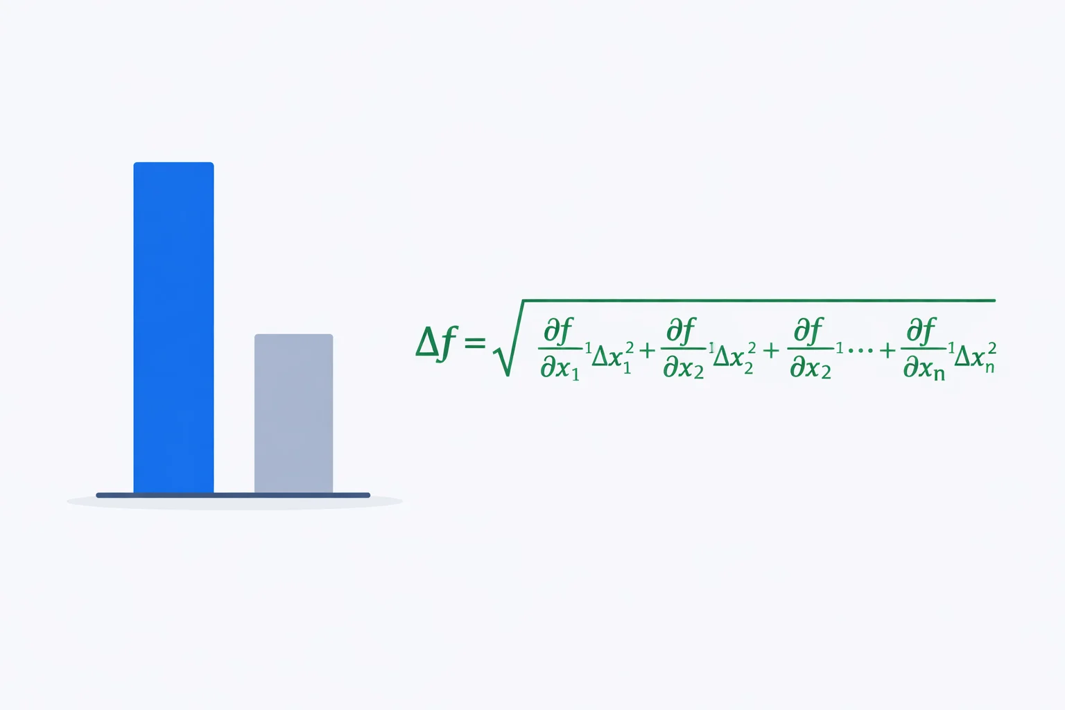
Every propagation shortcut descends from one parent equation. If a result R depends on measured quantities, the general rule is δR = √[ Σ (∂R/∂xᵢ · δxᵢ)² ] — take the partial derivative of R with respect to each variable, multiply by that variable's uncertainty, square, sum, and root. Differentiate a sum and the partial derivatives are just ±1, which collapses the formula to δR = √(δA² + δB²). Differentiate a product and the chain rule hands you the relative-error version. You almost never need to run the calculus by hand — the shortcuts below already bake it in — but knowing the rules share a single root explains why they look so different on the surface. For combining a whole formula by its exponents in one pass, the percent uncertainty calculator uses the maximum-error version of the same idea.
Sums and Differences: Combine Absolute Errors
When you add or subtract measurements, you combine their absoluteuncertainties — and it's combination for subtraction too, never cancellation. Lay a rod of 84.2 cm ± 0.1 cm end to end with one of 61.5 cm ± 0.1 cm. The total is 145.7 cm. Maximum error gives ±(0.1 + 0.1) = ±0.2 cm; quadrature gives ±√(0.1² + 0.1²) = ±0.14 cm. The minus sign in a difference applies only to the values: subtract those same rods and the length is 22.7 cm, but the uncertainty is still ±0.2 or ±0.14 cm. That's the subtraction trap — the result can shrink while the error doesn't, so a difference of two large, precise numbers can carry a shockingly large relative error.
Products and Powers: Combine Relative Errors
The moment a formula multiplies, divides, or raises to a power, you switch from absolute to relative uncertainties. Compute power from a current of 2.00 A ± 0.05 A and a voltage of 12.0 V ± 0.1 V. The current is good to 2.5%, the voltage to 0.83%. Maximum error adds them: 3.33%. Quadrature roots the squares: √(2.5² + 0.83²) = 2.63%. Multiply 24.0 W by either and you get ±0.80 W or ±0.63 W. You can watch the central value form in the electrical power calculator and then attach whichever error bar your course expects. Exponents ride along inside the relative term: a quantity raised to the power n contributes |n| × (δx/x), so squaring a measurement doubles its share and a square root halves it.
Maximum Error vs Quadrature, Side by Side
The two methods diverge faster as you add more terms, because quadrature's squaring increasingly favours the biggest contributor. Here's how four equal 2% terms combine under each rule as the count grows:
| Terms (each ±2%) | Maximum error (Σδ) | Quadrature (√Σδ²) | Quadrature is smaller by |
|---|---|---|---|
| 2 terms | 4.00% | 2.83% | 29% |
| 3 terms | 6.00% | 3.46% | 42% |
| 4 terms | 8.00% | 4.00% | 50% |
| 6 terms | 12.00% | 4.90% | 59% |
Notice the trend: by four terms, quadrature is already half the maximum-error figure, and the gap keeps widening. This is exactly why serious experimental work uses quadrature — the maximum-error rule becomes punishingly pessimistic once a calculation stacks up several independent inputs, quoting an error bar far wider than the data deserves.
Worked Example: Resistivity From Four Measurements
Resistivity is a great stress test because it folds four measurements into one formula: ρ = R·A/L = R·πd²/(4L), where R is resistance, d is wire diameter, and L is length. Say you measure R = 4.20 Ω ± 0.05 Ω, d = 0.500 mm ± 0.005 mm, and L = 1.000 m ± 0.002 m. The relative errors are 1.19% for R, 1.00% for d, and 0.20% for L — but d is squared, so its contribution is 2 × 1.00% = 2.00%.
Maximum error sums them: 1.19% + 2.00% + 0.20% = 3.39%. Quadrature roots the squares: √(1.19² + 2.00² + 0.20²) = √(1.42 + 4.00 + 0.04) = √5.46 = 2.34%. The diameter term, at 4.00 out of 5.46, owns 73% of the varianceall by itself — because it's both the largest relative error and the one that gets squared. Chasing a better ruler for L would be pointless; it contributes under 1% of the total error. Re-measuring d with a micrometer instead of calipers is the only change that actually tightens the result. Plug the four values into the calculator's product mode (with d at exponent 2) and the contribution table flags d for you automatically.
The Squaring Trick: Why One Term Usually Wins
Quadrature squares every contribution before summing, and squaring is brutally unfair to small numbers. A term that's one-third the size of the largest contributes only one-ninth as much to the variance. So in most real calculations a single measurement — the least precise one, or the one carrying the biggest exponent — dominates the final error, and everything else is a rounding correction. The practical payoff is a clear priority list: find the dominant term, improve that measurement, and ignore the rest. A common version shows up when you find gravitational acceleration from a pendulum: g depends on the period T squared, so the timing error gets doubled and almost always dominates the length error — which is why experimenters time many oscillations at once rather than a single swing.
When Quadrature Is the Wrong Choice
Quadrature isn't universally correct — it rests on the assumption that your errors are independent and random, and that assumption can fail. If two measurements share a systematic bias — say both lengths read with the same mis-zeroed ruler — those errors are correlated, not independent, and they really do add directly rather than in quadrature. A miscalibrated instrument that's always 2% high introduces a bias that no propagation rule for random error will catch; that's an accuracy problem, not a precision one. And if your course or exam board specifies the maximum-error method, use it regardless of what's statistically optimal — markers grade against their own rule. The methods also converge when one term dominates: if a single error is ten times any other, quadrature and maximum error agree to within a percent, so the choice stops mattering. The authoritative treatment of when each applies is the NIST reference on measurement uncertainty, which professional metrology labs follow.
Propagation Mistakes That Skew the Final Error
- Mixing absolute and relative in one step. Sums combine absolute errors; products combine relative ones. Work outward in stages — never feed a raw ± into a multiplication, or a percentage into a sum.
- Forgetting the exponent.A squared quantity contributes 2 × its relative error, and a cube contributes 3 ×. Drop the factor and you can halve a dominant term's real influence on the result.
- Subtracting the uncertainties when you subtract the values. Uncertainties always combine, never cancel. The minus sign belongs to the numbers, not their errors.
- Using quadrature on correlated errors. Quadrature assumes independence. Two readings sharing one biased instrument are correlated and should be added directly.
- Quoting too many digits. Round the uncertainty to one significant figure first, then trim the value to match. 2.3416 ± 0.0291 should read 2.34 ± 0.03.