Standard Deviation Calculator: Reading the Spread in Repeated Lab Measurements
You time a pendulum's swing six times and read 2.01, 1.98, 2.05, 1.99, 2.03, and 2.00 seconds off the stopwatch. Six tries, six different numbers — and none of them is wrong. The spread is real. It comes from your reaction time and the fuzziness of judging exactly when the bob crosses the mark, and your job is to turn that scatter into a single honest measure of reliability. That's what a standard deviation calculator does: it collapses a column of slightly disagreeing readings into one number that says how tightly your data clusters around its average. A small standard deviation means your technique was steady. A large one means either the quantity itself fluctuates or your method is noisy.
Five Stopwatch Readings That Won't Agree
Start with the average. The six timings sum to 12.06 s, so the mean period is 2.01 s. But the mean hides everything interesting — a set of readings of 2.01, 2.01, 2.01 has the same mean as 1.50, 2.01, 2.52, and those are wildly different measurements. Standard deviation is the number that separates the two cases. It answers "on average, how far does a single reading sit from the mean?" — not the plain average distance, but the root-mean-square distance, which weights the far-flung points more heavily.
For the pendulum data the deviations from 2.01 are 0.00, −0.03, +0.04, −0.02, +0.02, and −0.01 seconds. Square them, add them, and you get a sum of squares of 0.0034 s². That tiny number is the raw material for everything that follows. The whole game of standard deviation is taking that sum of squared misses, averaging it sensibly, and square-rooting back into the original units of seconds.
Building the Formula From the Mean Outward
The sample standard deviation is s = √( Σ(xᵢ − x̄)² ÷ (n − 1) ). Read it from the inside out and it's less intimidating than it looks. Subtract the mean x̄ from each reading xᵢ to get a deviation. Square each deviation so negatives don't cancel positives and so larger misses count for more. Add them all up — that's the Σ. Divide by n − 1, and take the square root to undo the squaring and land back in seconds.
Why square the deviations at all, instead of just taking their absolute values? Squaring does two useful things at once. It kills the sign problem cleanly, and it deliberately punishes outliers — a reading twice as far from the mean contributes four times as much to the sum. That sensitivity is a feature when you want to flag erratic data and a bug when one mistimed press distorts the whole result, a tension we'll come back to. The square root at the end is what keeps the answer in the same units as the data, so a spread in seconds reports in seconds, not seconds-squared. Seconds-squared is the variance — the standard deviation before you take the root.
Why Lab Data Almost Always Divides by n − 1
Here's the choice that trips up more students than the formula itself: do you divide by n or by n − 1? The pendulum data has six readings, so n = 6. Dividing the sum of squares 0.0034 by 6 gives the population standard deviation, 0.0238 s. Dividing by 5 instead gives the sample standard deviation, 0.0261 s. Same data, two answers that differ by about 10%.
For physics lab work you want the sample version, dividing by n − 1. The reasoning is subtle but worth getting: your six timings aren't the whole story — they're a small sample of the infinitely many timings you couldhave taken. When you measure spread around the sample mean rather than the unknown true mean, you systematically underestimate the real spread, because your data hugs its own average a little too closely. Dividing by n − 1 instead of n inflates the result just enough to cancel that bias. This is Bessel's correction, and its effect shrinks as n grows — at 30 readings the two divisors differ by under 2%, at 100 they're nearly identical. Reach for the population formula only when your data genuinely is the entire group: every lap time you ran today, every resistor in one sealed batch.
Standard Deviation Tells You Spread, Standard Error Tells You Confidence
This is the single most valuable distinction on the page, and most introductory courses rush past it. Standard deviation measures how scattered your individual readings are. Standard error of the mean (SEM) measures how well you've nailed down the average. They answer different questions, and mixing them up is a classic way to quote an uncertainty that's wrong by a factor of √n. The link is simple: SEM = s ÷ √n.
For the pendulum, s = 0.0261 s and n = 6, so SEM = 0.0261 ÷ √6 = 0.0107 s. You'd report the period as 2.010 ± 0.011 s, using the standard error, not the standard deviation. Why the smaller number? Because averaging six noisy readings gives a more trustworthy mean than any single reading — the noise partly averages out. Take more data and the SEM keeps shrinking even though the standard deviation barely changes. That asymmetry is the whole reason we repeat measurements.
| Standard deviation (s) | Standard error (SEM) | |
|---|---|---|
| Describes | Spread of individual readings | Uncertainty in the mean |
| Formula | √(Σ(x−x̄)²/(n−1)) | s ÷ √n |
| As n grows | Settles toward true spread | Keeps shrinking |
| Quote it when | Describing variability of the data | Stating ± on your final mean |
Once you have that standard error, it rarely stops there. If your period feeds into a calculation of g, you carry the uncertainty forward — that's a job for the error propagation calculator, which combines the standard errors of several measured quantities into the uncertainty of the final result.
The 68–95–99.7 Rule and What It Buys You
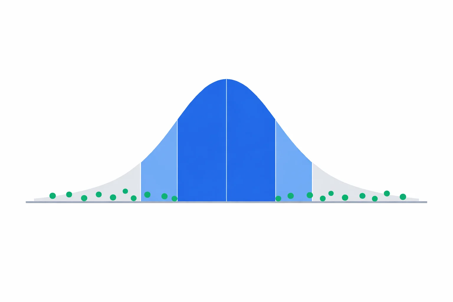
When repeated measurements scatter for purely random reasons, they pile up into a normal (bell-shaped) distribution, and the standard deviation marks off predictable slices of it. About 68% of readings land within one standard deviation of the mean, 95% within two, and 99.7% within three. This empirical rule is what makes the standard deviation a working tool rather than an abstract number — it lets you predict where the next reading should fall.
| Range | Fraction of data | Pendulum interval (s) |
|---|---|---|
| x̄ ± 1σ | 68.3% | 1.98 to 2.04 |
| x̄ ± 2σ | 95.4% | 1.96 to 2.06 |
| x̄ ± 3σ | 99.7% | 1.93 to 2.09 |
This is also where outlier-hunting gets a rule of thumb. A reading beyond ±3σ should happen roughly 3 times in 1000 by chance alone, so a single point that far out is far more likely a mistimed stopwatch than a genuine fluctuation. The dot plot in the calculator shades the ±1σ and ±2σ bands for exactly this reason — anything stranded outside them is asking for a second look.
Worked Example: The Pendulum Timings in Full
Let's run the six readings end to end so every step is visible. Data: 2.01, 1.98, 2.05, 1.99, 2.03, 2.00 s.
- Mean: (2.01 + 1.98 + 2.05 + 1.99 + 2.03 + 2.00) ÷ 6 = 12.06 ÷ 6 = 2.010 s.
- Deviations: 0.000, −0.030, +0.040, −0.020, +0.020, −0.010 s.
- Squared deviations: 0, 0.0009, 0.0016, 0.0004, 0.0004, 0.0001 — summing to 0.0034 s².
- Sample variance: 0.0034 ÷ (6 − 1) = 0.00068 s².
- Sample standard deviation: √0.00068 = 0.0261 s.
- Standard error: 0.0261 ÷ √6 = 0.0107 s.
So the final reported period is 2.010 ± 0.011 s. Notice how the uncertainty (0.011 s) is much smaller than the spread of the raw data, which ranged across 0.07 s from fastest to slowest. That gap is the payoff of repetition. If you only need the spread of the data — say you're characterising how noisy your timing technique is — you'd quote the 0.026 s standard deviation instead. Once you have the mean and its error, compare it to the accepted value with the percent error calculator to judge accuracy alongside precision.
When the Standard Deviation Quietly Misleads
The standard deviation assumes your scatter is roughly symmetric and random, and it breaks down when that assumption fails. Skewed data is the first trap: if your readings have a long tail on one side — common with timing data, where you can be very late but never negative — the standard deviation overstates the typical spread and the mean sits off-centre. The bell-curve picture, and the 68–95–99.7 rule with it, no longer holds.
The second trap is small n. With only three or four readings the standard deviation is a shaky estimate that lurches around with every new data point, and a lone outlier can double it. The third is reading too much into a tiny spread. A standard deviation of zero — six identical readings — doesn't mean your measurement is perfect; it usually means your instrument can't resolve the variation, like timing a fast event with a stopwatch that only reads whole seconds. A small standard deviation says your readings agree with each other, not that they agree with reality. For that second question — how close the mean lands to the true value — you need accuracy, not precision, and the standard deviation is silent on it.
Mistakes That Cost Lab Marks
- Dividing by n when you should use n − 1.Check your handheld calculator's mode — many default to the population formula (σn). For small samples this understates the spread by a noticeable margin.
- Reporting the standard deviation as the uncertainty in the mean. The uncertainty on your average is the standard error, s ÷ √n, which is smaller. Quoting the full standard deviation as your ± inflates your error bars by a factor of √n.
- Forgetting to square-root. The variance is in squared units. If your answer looks suspiciously small and is labelled s², you stopped one step early.
- Deleting an inconvenient outlier. A point outside ±2σ is a flag to investigate, not a licence to delete. Reject a reading only with a documented physical reason, then recompute — and say so in your write-up.
- Over-reporting digits.A standard deviation from six readings doesn't justify five significant figures. Round it sensibly with the significant figures calculator before it goes in the report.
For the formal treatment of how repeated readings define a measurement uncertainty, the NIST guide to evaluating measurement uncertainty is the authoritative reference, and it leans on exactly the standard deviation and standard error you've just calculated.