Squeeze a Garden Hose, Watch Pressure Drop: Solving Problems with Bernoulli’s Equation
You're watering the garden and you slide your thumb across the hose opening. The stream narrows, shoots farther, and the water feels faster against your hand. But here's the part most people miss: the Bernoulli's equation calculator above would show you that the static pressure inside the hose at the constriction actually dropped. Faster fluid, lower pressure. That tradeoff — kinetic energy up, pressure energy down, total unchanged — is the entire content of Bernoulli's equation, and it governs everything from carburetor throats to airplane pitot tubes.
The Garden Hose Problem
Let's turn that garden hose observation into numbers. A standard ¾-inch garden hose has an inside diameter of about 19 mm, giving a cross-sectional area of 2.84 cm². Municipal water pressure delivers roughly 3.5 bar (350,000 Pa) at your faucet, and at a typical flow rate of 15 L/min the water moves through the hose at about 0.88 m/s. Nothing dramatic.
Now you squeeze the opening to 8 mm diameter (area = 0.50 cm²). Continuity demands that the same 15 L/min passes through a smaller area, so velocity jumps to 0.88 × (2.84 / 0.50) = 5.0 m/s. Bernoulli's equation says the static pressure at the constriction drops by ½ρ(v₂² − v₁²) = 0.5 × 998 × (25 − 0.77) ≈ 12,100 Pa. That's about 0.12 atm — modest, but measurable. The pressure energy didn't vanish; it converted into the kinetic energy that launches the stream across your yard.
Three Energy Terms, One Constant Sum
Bernoulli's equation along a streamline is:
P + ½ρv² + ρgh = constant
Each term has units of pascals (Pa = N/m² = J/m³), so the equation is really an energy-per-volume budget. Pis the static pressure — the energy stored in the fluid's random molecular motion pressing on pipe walls. ½ρv²is the dynamic pressure — kinetic energy of bulk flow per unit volume. ρghis the hydrostatic term — gravitational potential energy per unit volume, identical to the gravitational potential energy you'd calculate for a solid mass, just expressed per cubic meter instead of per kilogram.
The equation applies when three assumptions hold: the fluid is incompressible(constant ρ), the flow is steady (no time-varying changes), and viscous losses are negligible. Water in short, smooth pipes satisfies all three comfortably. Air at low speeds works too. Honey in a long capillary tube — not so much.
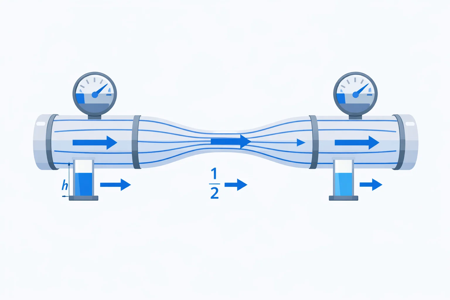
Worked Example: A Pipe Constriction
A horizontal water pipe narrows from 80 mm to 40 mm diameter. The pressure in the wide section is 250 kPa gauge, and the flow velocity there is 1.5 m/s. What's the pressure in the narrow section?
Step 1 — find v₂.The continuity equation (A₁v₁ = A₂v₂) gives v₂ = v₁ × (d₁/d₂)² = 1.5 × (80/40)² = 1.5 × 4 = 6.0 m/s. The diameter halved, so the area quartered, so velocity quadrupled.
Step 2 — apply Bernoulli (h₁ = h₂, so the ρgh terms cancel).
P₂ = P₁ + ½ρ(v₁² − v₂²)
P₂ = 250,000 + 0.5 × 998 × (1.5² − 6.0²)
P₂ = 250,000 + 499 × (2.25 − 36)
P₂ = 250,000 − 16,841
P₂ = 233,159 Pa ≈ 233.2 kPa
The pressure dropped by about 16.8 kPa — roughly 6.7% — because kinetic energy absorbed the difference. If you plugged these numbers into the calculator above in Venturi mode (80 mm wide, 40 mm narrow, 250 kPa, 1.5 m/s), you'd get exactly the same answer. Try it.
The Venturi Effect and Where You've Already Seen It
The Venturi effect is Bernoulli's equation applied to a deliberate constriction. Speed goes up, pressure goes down, and engineers exploit that pressure drop for measurement, mixing, and suction:
- Carburetor throats— air accelerates through the Venturi, dropping pressure enough to draw fuel from a reservoir through a small jet. A typical carburetor throat diameter of 28 mm with a 36 mm main bore creates a velocity ratio of about 1.65× and a pressure drop of roughly 2–5 kPa at idle, increasing with throttle opening.
- Aspirator pumps— lab water aspirators run tap water through a constriction to generate suction of 10–25 kPa below atmospheric, enough for basic vacuum filtration.
- Venturi meters— the gold standard of flow measurement. By measuring the pressure difference between wide and narrow sections, you can back-calculate flow rate to ±1% accuracy with no moving parts and minimal permanent pressure loss (5–15% of the differential reading).
- Spray bottles— squeezing the trigger pushes air across a narrow tube opening, creating a low-pressure zone that draws liquid up the dip tube.
Torricelli's Shortcut: How Fast Does a Tank Drain?
Point Bernoulli's equation at the surface of an open tank (Point 1: atmospheric pressure, velocity ≈ 0, height h) and at a small drain hole at the bottom (Point 2: atmospheric pressure, velocity v, height 0). The P terms cancel, the v₁ term vanishes, and you get:
v = √(2gh)
This is Torricelli's theorem, published in 1643, and it's identical to the speed of an object in free fall from height h. A 2-meter tank drains at v = √(2 × 9.81 × 2) = 6.26 m/s — about 22.5 km/h. A 50-meter water tower gives 31.3 m/s (113 km/h), which is why fire hydrants can knock you off your feet.
The counterintuitive part: velocity depends on √h, not h. To double the exit speed, you need four times the height. This square-root relationship explains why draining the last 10% of a tank feels painfully slow — at one-tenth the original height, exit velocity has dropped to √(0.1) ≈ 0.316 times its initial value, or about 32% speed.
When Bernoulli's Equation Gives Wrong Answers
Bernoulli's equation fails silently when its assumptions break. Here's when to stop trusting it:
| Assumption Violated | What Happens | Use Instead |
|---|---|---|
| Viscous fluid (honey, oil in long pipes) | Friction converts kinetic energy to heat; actual downstream pressure is lower than predicted | Bernoulli + Darcy-Weisbach head loss |
| Compressible flow (air above Mach 0.3) | Density changes significantly; ρ is no longer constant | Compressible Bernoulli with isentropic relations |
| Turbulence / eddies | Energy dissipates in vortices; total pressure decreases along the streamline | Navier-Stokes equations (CFD) |
| Flow crosses streamlines (curved paths, mixing) | Bernoulli only applies along a single streamline, not across them | Euler's equation normal to streamlines |
| Unsteady flow (water hammer, pulsating pumps) | Time-dependent pressure waves that Bernoulli ignores | Unsteady Bernoulli with ∂φ/∂t term |
A reliable rule of thumb: if your Reynolds number is below 4,000 (laminar flow) and the pipe run is short relative to the diameter, Bernoulli's equation gives answers within 5% of reality. For a 50 mm pipe carrying water at 2 m/s, Re ≈ 100,000 — that's well into turbulent territory, but in short sections with smooth walls, the ideal Bernoulli prediction still lands close. In a 100-meter pipe run at the same speed, friction losses accumulate and you need Darcy-Weisbach corrections.
Pressure–Velocity Reference Table for Common Pipe Scenarios
This table shows how fluid density and velocity interact to determine dynamic pressure (½ρv²) — the term that drives Bernoulli's pressure changes:
| Scenario | ρ (kg/m³) | v (m/s) | ½ρv² (Pa) | Equivalent |
|---|---|---|---|---|
| Residential water pipe | 998 | 1.5 | 1,123 | 0.011 atm |
| Fire hose nozzle | 998 | 20 | 199,600 | 1.97 atm |
| Oil pipeline | 880 | 3 | 3,960 | 0.039 atm |
| Car at highway speed (air) | 1.225 | 30 | 551 | 0.005 atm |
| Hurricane-force wind | 1.225 | 70 | 3,001 | 0.030 atm |
| Pitot tube at 250 km/h | 1.225 | 69.4 | 2,952 | 0.029 atm |
Notice the enormous difference between water and air at the same velocity. At 3 m/s, water's dynamic pressure (3,960 Pa) is 815× higher than air's at the same speed (4.86 Pa), because ρ for water is 815× larger. This is why hydraulic systems use liquid — the energy density per unit volume is dramatically higher.
Three Errors That Lose Points on Every Exam
Forgetting gauge vs. absolute pressure.Bernoulli's equation works with both, but you must be consistent. If P₁ is gauge, P₂ must be gauge. Mixing gauge and absolute introduces a 101,325 Pa error — larger than most dynamic pressure terms in typical homework problems, so the answer comes out wildly wrong.
Using the wrong height datum.The ρgh terms require a consistent reference level. If h₁ is measured from the floor and h₂ from the ceiling, the equation won't conserve energy. Pick one reference point (usually the lowest point in the problem) and measure all heights from there.
Ignoring the continuity equation.Bernoulli alone has six unknowns (P₁, v₁, h₁, P₂, v₂, h₂) and only one equation. You almost always need continuity (A₁v₁ = A₂v₂) to eliminate one velocity. Students who try to solve Bernoulli problems without continuity end up with two unknowns and one equation — unsolvable. Write both equations side by side before you start plugging in numbers.