What is marginal physical product in economics?

Marginal physical product (MPP) is the additional output produced when one more unit of a variable input (like labor) is added while all other inputs remain constant. It is calculated as the change in total product divided by the change in input quantity: MPP = ΔTP / ΔL. MPP is a core concept in production theory and helps firms determine the optimal number of workers or machines to employ.

How do you calculate marginal physical product of labor?

To calculate the marginal physical product of labor, subtract the previous total output from the new total output after adding one more worker. For example, if 3 workers produce 90 units and 4 workers produce 110 units, the MPP of the 4th worker is 110 minus 90, which equals 20 units. The formula is MPP = ΔTP / ΔL, where ΔTP is the change in total product and ΔL is the change in labor input.

What is the law of diminishing marginal returns?

The law of diminishing marginal returns states that as you add more units of a variable input to a fixed input, the marginal physical product of each additional unit will eventually decrease. For example, adding a 5th worker to a small kitchen might increase output by 15 meals, but a 6th worker might only add 8 meals because the workspace becomes crowded. This law applies in the short run when at least one factor of production is fixed.

What is the difference between marginal product and average product?

Marginal product measures the additional output from one more input unit, while average product measures total output divided by the total number of input units. For example, if 5 workers produce 100 units total, the average product is 20 units per worker, but the marginal product of the 5th worker might only be 12 units. When marginal product equals average product, average product is at its maximum — this is a key relationship in production economics.

Can marginal physical product be negative?

Yes, marginal physical product can become negative. This happens when adding another unit of input actually decreases total output. For example, hiring too many workers in a small factory can lead to overcrowding, confusion, and lower total production. Negative MPP occurs in Stage III of production, and no rational firm would operate in this range because reducing inputs would actually increase output.

How is marginal physical product used to determine optimal hiring?

Firms compare the marginal physical product of labor with the cost of hiring to find the profit-maximizing number of workers. The optimal hiring point is where the value of marginal product (MPP multiplied by the product price) equals the wage rate. If MPP times price exceeds the wage, hiring another worker increases profit. If it falls below the wage, the firm should reduce workers.

What are the three stages of production?

Stage I runs from zero input to where average product reaches its maximum — MPP is above APP and both are rising. Stage II runs from maximum average product to where marginal product reaches zero — this is the economically rational stage where firms should operate. Stage III begins where marginal product becomes negative, meaning total product is actually declining. No firm should produce in Stage III.

What is the relationship between MPP and the production function?

The marginal physical product is the slope of the total product curve at any given input level. When the production function is expressed as TP = f(L), the MPP equals the first derivative dTP/dL. A steeper production curve means higher MPP, while a flattening curve indicates diminishing marginal returns. The shape of the production function directly determines whether MPP is increasing, decreasing, or negative.

Marginal Physical Product Calculator

L	TP	MPP	APP	Stage
0	0.0	—	—	I
1	10.0	10.0	10.00	I
2	25.0	15.0	12.50	I
3	45.0	20.0	15.00	I
4	60.0	15.0	15.00	II
5	70.0	10.0	14.00	II
6	75.0	5.0	12.50	II
7	73.0	-2.0	10.43	III

Learning how to calculate marginal physical product is one of the most important skills in production economics. Marginal physical product (MPP) tells you exactly how much additional output you gain by adding one more unit of input — whether that's an extra worker on a factory floor, another machine in a warehouse, or an additional acre of farmland. This calculator instantly computes MPP, average physical product, and identifies the point of diminishing returns so you can make smarter production decisions.

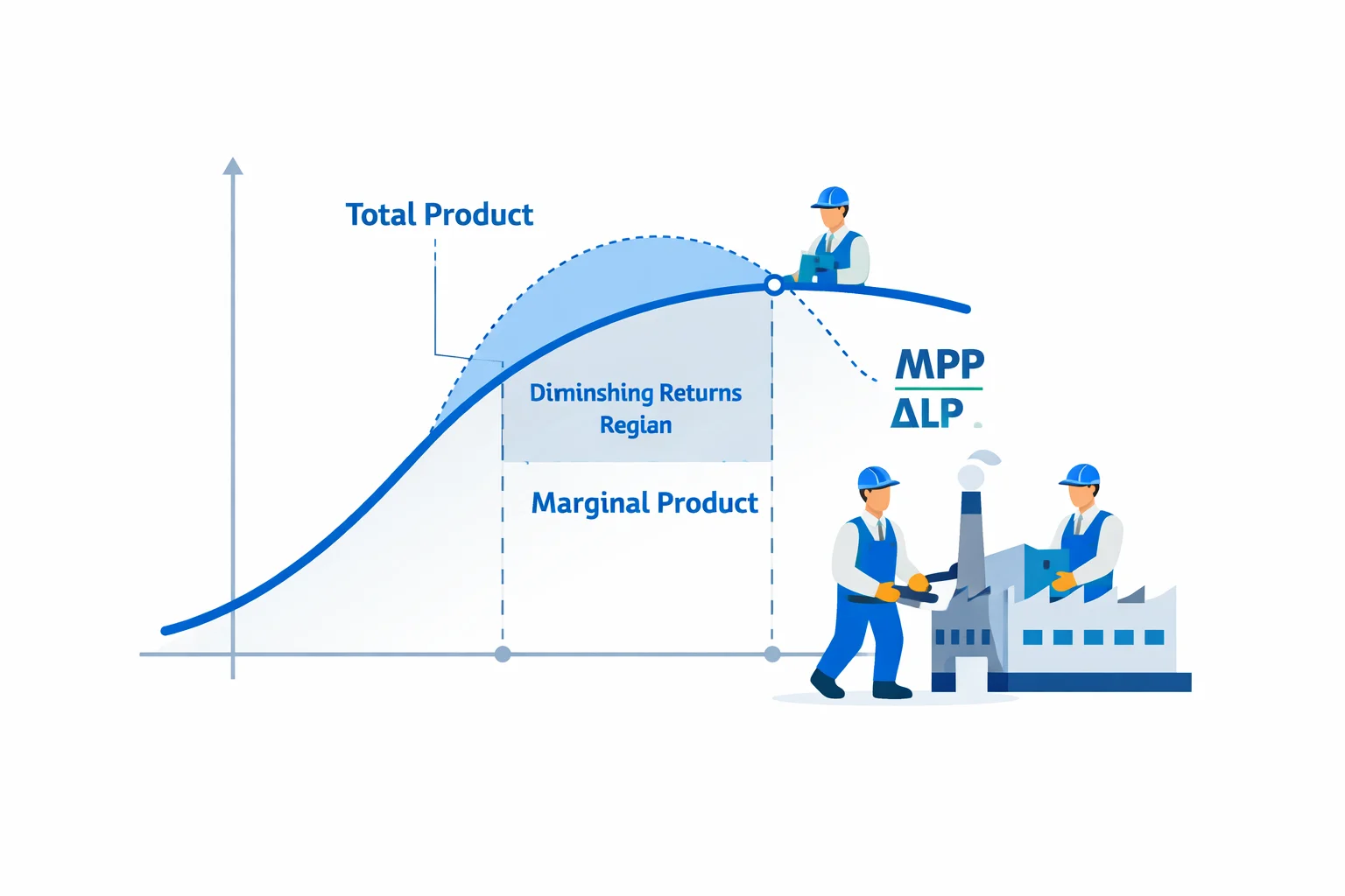
Marginal physical product diagram showing total product curve, diminishing returns region, and MPP formula with production function analysis

What Is Marginal Physical Product?

Marginal physical product (MPP) measures the change in total output that results from employing one additional unit of a variable input, holding all other inputs constant. In simpler terms: if you hire one more worker and your factory output goes from 100 units to 115 units, the marginal physical product of that worker is 15 units.

MPP is also called marginal product (MP) or marginal physical product of labor (MPP_L) when labor is the variable input. It sits at the heart of production theory because it directly determines how profitable each additional unit of input is. Firms use MPP to decide how many workers to hire, how much capital to deploy, and when adding more input stops being worthwhile.

The Marginal Physical Product Formula

The formula for marginal physical product is straightforward:

MPP = ΔTP / ΔL

Where ΔTP is the change in total product (output) and ΔL is the change in the variable input (labor). When labor increases by exactly one unit, MPP simply equals the new total product minus the old total product.

For continuous production functions like the Cobb-Douglas function TP = A × L^b, the marginal product is the first derivative of the production function with respect to the variable input:

MPP = dTP/dL = A × b × L^(b−1)

When the exponent b is less than 1, each additional unit of labor produces less than the previous one — this is the mathematical foundation of diminishing returns.

Worked Example: Calculating MPP Step by Step

Suppose a small bakery tracks its daily bread loaf output as it adds workers:

Workers (L)	Total Loaves (TP)	MPP	APP
0	0	—	—
1	20	20	20.00
2	50	30	25.00
3	90	40	30.00
4	120	30	30.00
5	140	20	28.00
6	150	10	25.00
7	148	−2	21.14

Step 1: The 3rd worker increases output from 50 to 90. MPP = 90 − 50 = 40 loaves. This is the peak MPP.
Step 2: The 4th worker increases output from 90 to 120. MPP = 120 − 90 = 30 loaves. Diminishing returns have begun.
Step 3: The 7th worker decreases total output from 150 to 148. MPP = 148 − 150 = −2 loaves. The kitchen is overcrowded — Stage III.

Notice how APP peaks at 30.00 when L = 3 and L = 4. At worker 4, MPP equals APP — this marks the transition from Stage I to Stage II and is the maximum point of average efficiency.

The Three Stages of Production

Every production process with a fixed input passes through three distinct stages as the variable input increases:

Stage I (Increasing Returns): MPP may rise or fall, but APP is still increasing. The variable input is being underutilized relative to the fixed input. In the bakery example, Stage I runs from workers 1 through 3.
Stage II (Diminishing Returns): APP is declining and MPP is positive but falling. This is the rational stage of production where firms should operate. In the bakery, Stage II runs from workers 4 through 6.
Stage III (Negative Returns): MPP is negative — adding more input actually reduces total output. Worker 7 in the bakery pushes production into Stage III. No rational firm operates here.

Understanding which stage your production is in helps you avoid both underinvestment (Stage I) and overinvestment (Stage III). If you're analyzing how capital equipment relates to worker productivity, try our physical capital per worker calculator to see the K/L ratio in action.

MPP vs. Average Physical Product (APP)

While MPP measures the additional output from the last unit of input, average physical product (APP) measures the output per unit across all inputs: APP = TP / L. Their relationship follows a predictable pattern:

When MPP > APP, average product is rising (adding above-average workers pulls the average up)
When MPP = APP, average product is at its maximum
When MPP < APP, average product is falling (adding below-average workers drags the average down)

Think of it like a student's GPA: if your next exam score (marginal) is higher than your current GPA (average), your GPA rises. If it's lower, your GPA falls. The crossover point — where MPP equals APP — is a critical landmark in production analysis.

Understanding Diminishing Marginal Returns

The law of diminishing marginal returns states that as a firm adds more of a variable input to fixed inputs, the marginal product of the variable input eventually declines. This is not a theory — it's an empirical regularity observed across virtually every industry.

Why does it happen? Because the fixed input becomes a bottleneck. A bakery with 2 ovens can keep adding bakers, but eventually those bakers are waiting for oven time. A farm can add workers, but the land area is fixed. The additional workers have less and less of the fixed resource to work with.

Key numbers to watch for: diminishing returns typically set in after MPP has peaked. In the Cobb-Douglas production function TP = A × L^b, diminishing returns occur whenever b < 1. With b = 0.7 (a common empirical estimate for labor), a firm with A = 10 would see MPP drop from 7.00 at L = 1 to 4.31 at L = 5 and 3.44 at L = 10 — a 51% decline in marginal productivity.

Common Mistakes When Calculating MPP

Confusing MPP with APP: MPP is the change in output, not the average output per worker. Using APP when you need MPP leads to incorrect hiring decisions.
Forgetting to hold other inputs constant: MPP is only valid when you change one input at a time. If you add 2 workers AND buy a new machine, you can't attribute the output change solely to labor.
Ignoring negative MPP: Some students assume MPP cannot be negative. It absolutely can — and recognizing negative MPP is critical because it means you should reduce the input, not increase it.
Applying MPP to long-run decisions: MPP is a short-run concept (at least one input is fixed). In the long run, all inputs are variable and you should use returns to scale analysis instead. For analyzing how scale affects productivity across different production scenarios, consider using the AP Physics 1 score calculator approach of breaking complex inputs into component sections.

Real-World Applications of Marginal Product

MPP is not just a textbook concept — it drives real business and policy decisions every day:

Hiring decisions: A restaurant compares the MPP of an additional chef (measured in meals per shift) to the wage cost. If the chef's MPP multiplied by revenue per meal exceeds their wage, hiring is profitable.
Agricultural planning: Farmers use MPP to determine the optimal amount of fertilizer. Adding 50 kg of fertilizer per hectare might increase wheat yield by 400 kg, but the next 50 kg might only add 200 kg — classic diminishing returns.
Factory staffing: A car manufacturer running 2 shifts at 80% capacity calculates the MPP of adding workers versus adding a 3rd shift. The fixed capital (assembly line) constrains how many workers are productive.
Sports analytics: Teams analyze the marginal contribution of each additional player dollar spent. A $30M player might add 5 wins, but a $50M player might only add 6 wins — the MPP of salary spending diminishes. You can explore similar rate-of-change analysis with a capital per worker calculator to see how capital deepening affects output.

When to Use This Calculator

This marginal physical product calculator is built for students, economists, and business analysts who need to:

Complete microeconomics homework or exam prep on production theory and diminishing returns
Analyze real production data to find the point of diminishing returns and the optimal input level
Explore how Cobb-Douglas production function parameters affect MPP, APP, and total product
Determine which stage of production a firm is operating in (Stage I, II, or III)
Compare marginal product to average product and understand when each metric matters most
Make data-driven hiring or resource allocation decisions by quantifying the output impact of each additional unit

Switch between Data Table Mode for real-world production data and Production Function Mode for theoretical analysis. Both modes instantly calculate MPP, APP, total product, and production stages so you can focus on understanding the economics rather than crunching numbers.

Marginal Physical Product Calculator